I love gadgets! Especially electronic devices. Measuring devices, in particular, are pretty irresistible to me. And thus, I own quite number of them to measure anything that may cross my path. Among them plenty of things for measuring distances/thickness/...: Rulers, tape measures, calipers, micrometers, laser tape measures and a laser rangefinder.

The last two may seem identical to the uninitiated reader but they serve different purposes. The laser tape measure excels at measuring things around the house and workshop at millimeter precision while the range finder is designed for much larger scales – several hundred meters/yards outdoors to an accuracy of less than a meter. E.g. on the golf course, while hiking, or just for fun.

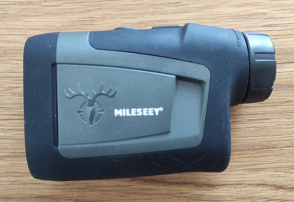
The range finder I have is of far eastern provenance and the specific model is called MILESEEY PF210 hunting. You can find it for less than 100 Euros.

From the data sheet:

Parameter	Value
Measurement range	3 – 800m
Accuracy	±0.5m + 0.01 digits
optic magnification	6x

But specs can be misleading, especially with cheap tools, so I am keen to dig deeper and find out how well it really performs. But what does it actually measure? These:

• Distance (line of sight)
• Slope
• Horizontal distance
• Height above instrument level
• Height difference between two points
• Speed

It also features a special rain/fog mode that will scan the distance and keep the largest distance measured.

The device can directly determine distance by the time of flight method and slope using a digital sensor similar to those found in modern smartphones or the popular bevel boxes. The rest is basic trigonometry.

In this analysis, we will focus on horizontal distance.

How to determine quality of such a device?

The quality of a measuring device is determined by many factors:

1. Precision (reproducibility)
2. Accuracy (trueness)
3. Interference (e.g. day/night, direct sunlight, temperature, rain, ...)
4. Measurement range (min/max)
5. Linearity
6. Acquisition time
7. ...

Let's have a closer look at the first two.

Precision

Precision is the measurement repeatability – i.e. if we repeat the same measurement over and over again, how well do they agree? Ideally, they should be identical but in practice you will most likely see some degree of variation between measurements.

There are many different levels/factors to consider in determining precision:

• Immediate repetition (within run precision)
• Different measurement runs, e.g. after turning the tool off and on. (between run precision)
• On separate days (between day precision)
• When operated by different people (between operator precision)
• Using different instruments of the same type and model (between instrument precision)
• When used at different sites (between site precision)

I don't feel like analyzing all of the above so this is my experiment plan:

• 10 different distances (groups)
• 10 measurements for each group
• Try and cover the measurement range (3-800m) as good as possible

100 single measurements all together. I will collect data in a spreadsheet and store it in csv format for easy analysis. I'm European, so all values are given in meters.

First, let's plot the data by group. The blue line indicates the group mean.

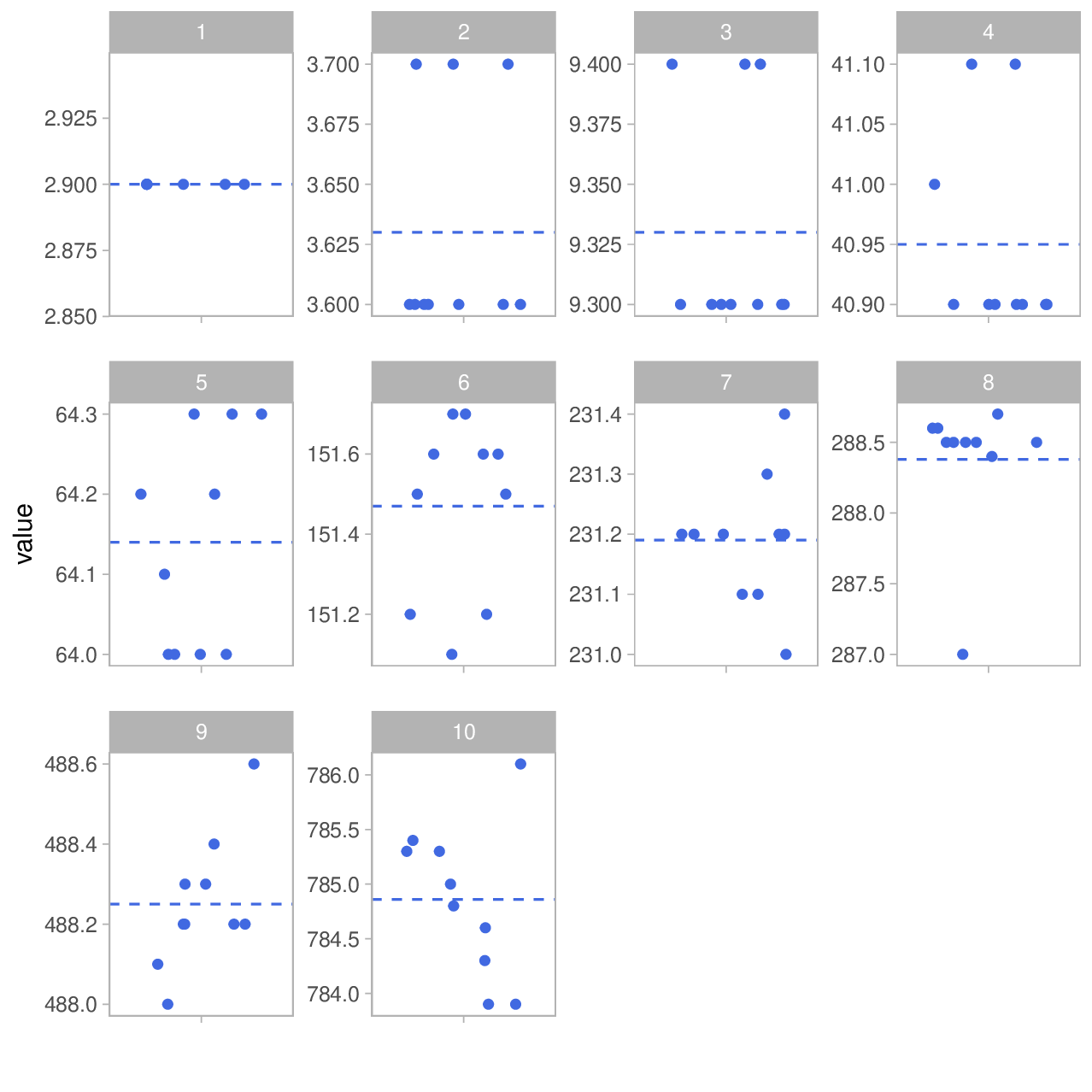
So we managed to cover a distance range from 2.9 to ≈785m. Excellent. If you paid close attention, you will probably wonder how our smallest distance can be 2.9m when the instrument's range starts at 3 m. The reason is that the direct distance actually was ≥3m but I tilted the instrument slightly up or down resulting in a lower horizontal distance. Actually, we are missing a few data points in this group as some measurements failed due to results below the lower limit.

In order to get a better impression of the deviation from the group mean, let's slightly change the plot and show something else:

I.e. the y-axis now shows the deviation from the group mean which is shown in the headers of the mini plots:

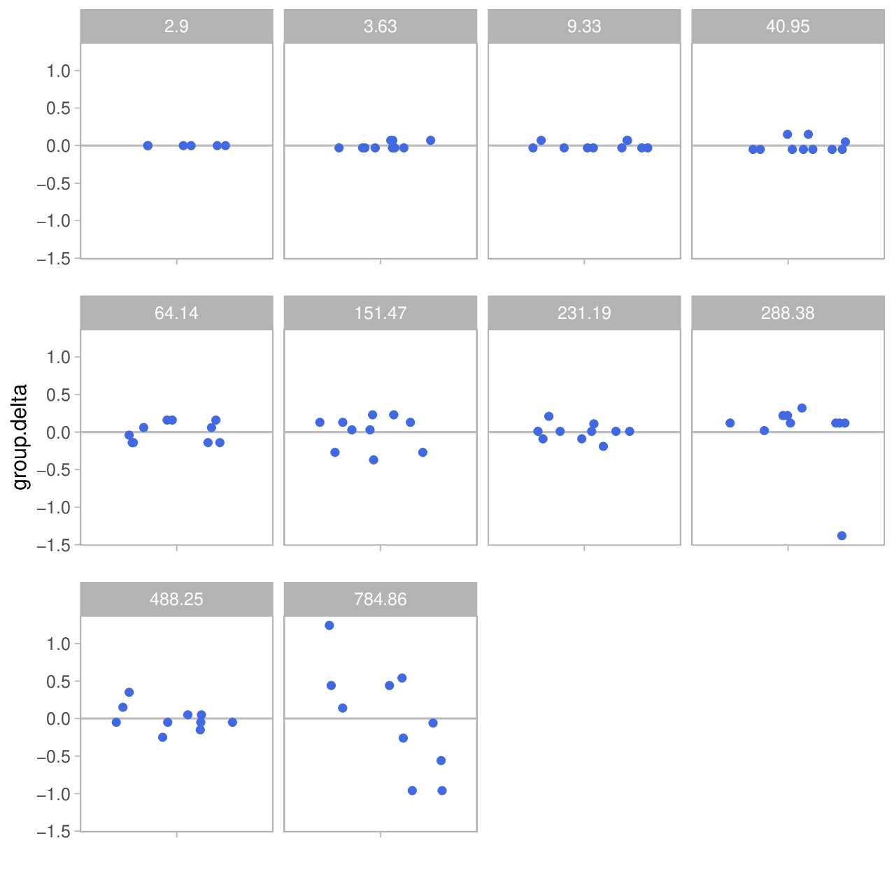
As you can see, the absolute deviation is pretty small at lower distances – almost invisible. But it increases with the measured distance until we get deviations up to almost 1 meter at ≈800m.

In addition, it may be interesting to look at the relative deviation (\(\Delta\)), instead – shown in percent on the y-axis:

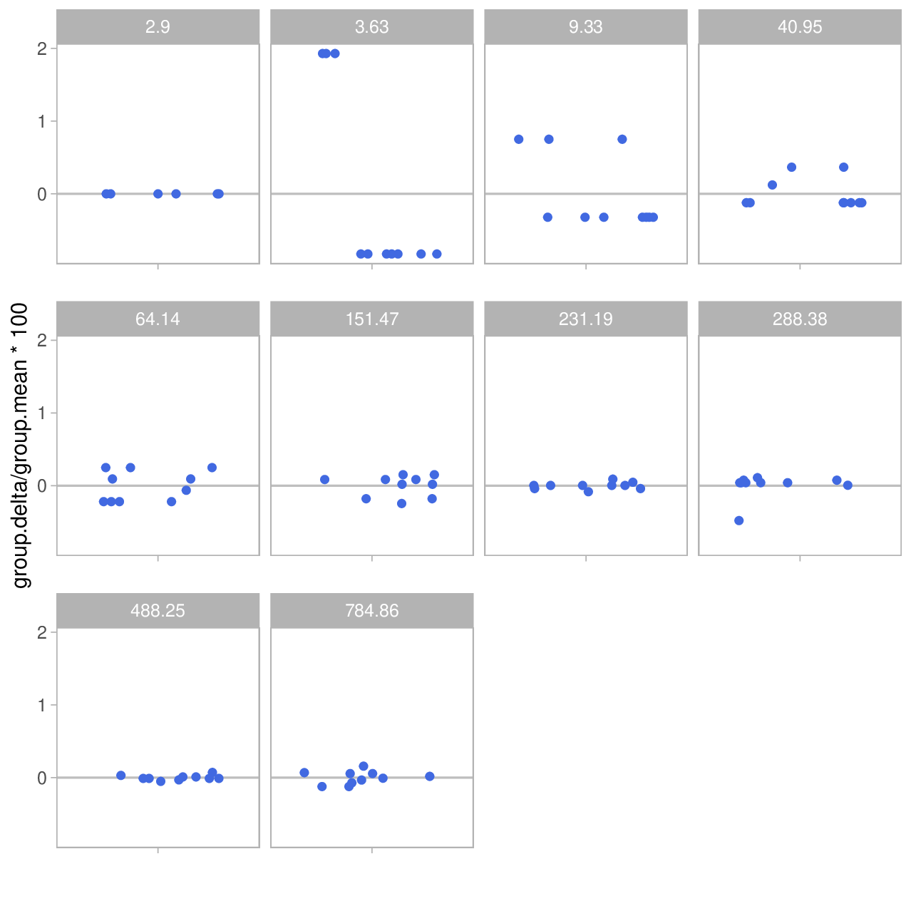
And now we see the opposite of the relative deviation: As the distance grows, relative deviation decreases: starting at ±1 or 2% at the lower end it goes down to fractions of a percent at the higher end of the range.

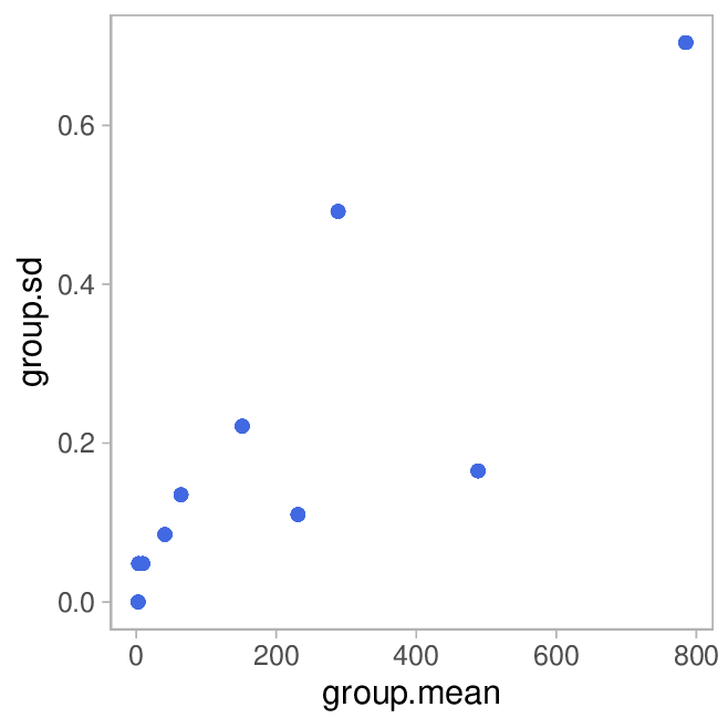
In order to quantify the precision, we can now calculate standard deviation (SD) in each group and the coefficient of variation (CV) which is given as

So it's the standard deviation normalized to the measurement value. That makes sense, because for many measurements, the SD increases with the measured value. The plot shows CV in percent on the y-axis:

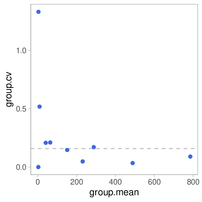
The dashed line indicates the median CV.

By and large, I am pretty happy with the precision observed.

Accuracy

So let's get to the second aspect – accuracy, aka trueness. While precision was concerned with how well repeated measurements would agree, accuracy is about how close our measurements are to the true value, on average. Investigating this is a bit more demanding than precision, because we now need reference values that represent the true distance. Given the distance range, things like a tape measure are clearly out as a reference method. My solutions is using online maps. Google maps has measuring capabilities and so does the official geography portal of the state of Bavaria – Bayern-Atlas. Except for two cases, I used that source by manually setting flags on the map and getting the distance value from the platform.

Now, these reference values aren't perfect, either. Errors and imprecisions in the map data are one potential problem, manual accuracy in setting the flags is another source of error. So one should keep this in mind when interpreting the results.

In addition, using the rangefinder can introduce further errors when you are not standing perfectly at the correct position or pointing the device slightly left/right of the spot that you marked in the map. Both effects reduce the agreement between both methods.

My experiment comprises 20 measurements with the range finder (\(value\)) accompanied by their respective reference values (\(ref\)). Now we plot the values over the references and get this:

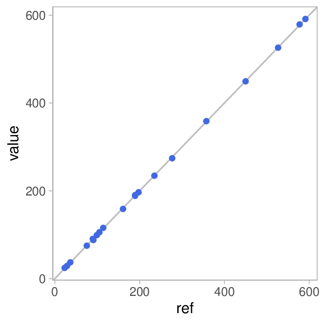
The grey diagonal line represent perfect agreement. As you can see, our data points are almost perfectly located on that line. And the correlation coefficient agrees with that assessment:

If we fit a linear model, we get

Almost perfect!

In order to zoom in on the deviations, we will add a Bland-Altman Plot. I.e. we show the difference between measured value and reference (\(value-ref\)) on the y-axis and the mean of the two on the x-axis (\((value + ref)/2\)). This makes it much easier to see the deviation depending on the distance measured:

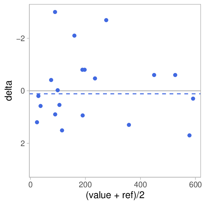
Again, the grey line indicates perfect agreement (\(\Delta = 0\)) and the dashed blue line is the mean deviation (bias)

Finally, we add a variation of the plot by showing the relative deviation (in percent) instead of the absolute difference.

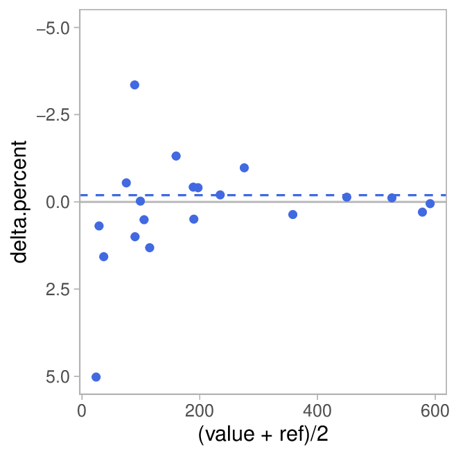
Comparing the two graphs is quite interesting: While the absolute deviation appears pretty constant across the range, this results in large relative errors for small distances while they become miniscule for larger distances.

Conclusion

I am pretty happy with the performance of my range finder. I certainly don't need more than this. It would have been interesting to also evaluate speed measurements but good reference values are much harder to generate in that case. Maybe later in a separate post.